RVT default module
This example notebook shows how the rvt.default module can quickly calculate or save any rvt visualization.
This notebook is suitable for beginner python users.
Before you start
You’ll need a DEM to work through this notebook.
Download the test data from Getting started, or have some of your own data ready to work with.
Save your data in a directory called test_data. You’ll need to set a path to this test data in cell [2].
Working with visualization parameters
To calculate a visualization we need to use visualization parameters (e.g. hillshade sun azimuth).
The default module has the rvt.default.DefultValues() class. All visualization parameters are stored as attributes of this class.
This class also contains methods to calculate the numpy array of a specific visualization, or to calculate and save a specific visualization as a GeoTIFF. All methods use class atributes (or set parameters).
For get methods we need the DEM numpy array, for save methods we need the DEM path.
If you call a save method for a specific visualization (e.g. default.save_hillshade()) it will be saved in the DEM directory (dem_path). To change the output directory, input the output directory as a string in custom_dir (save methods parameter).
Save methods also have two boolean parameters: save_float and save_8bit. If save_float is True, the method will save the visulization as float. If save_8bit is True, the method will bytescale visualization (0-255) and save it. Both can be True, if you want to save both.
Ok, let’s import the required modules:
[1]:
import matplotlib.pyplot as plt
import rvt.default
To get the visualization array we need to input the DEM numpy array.
We will use the default module function get_raster_arr() to read it.
[2]:
dem_path = r"../test_data/TM1_564_146.tif" # set path to your dem
[3]:
dict_dem = rvt.default.get_raster_arr(dem_path)
[4]:
dem_arr = dict_dem["array"] # numpy array of DEM
dem_resolution = dict_dem["resolution"]
dem_res_x = dem_resolution[0] # resolution in X direction
dem_res_y = dem_resolution[1] # resolution in Y direction
dem_no_data = dict_dem["no_data"]
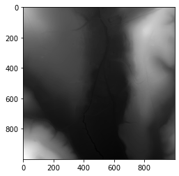
plt.imshow(dem_arr, cmap='gray') # show DEM
[4]:
<matplotlib.image.AxesImage at 0x17d9c68c888>
Create rvt.default.DefaultValues() class:
[5]:
default = rvt.default.DefaultValues() # we created instance of class and stored it in default variable
Slope
Set parameters:
[6]:
default.slp_output_units = "degree"
Calculate numpy array:
[7]:
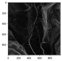
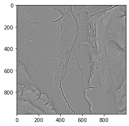
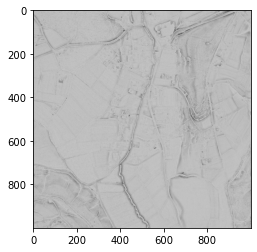
slope_arr = default.get_slope(dem_arr=dem_arr, resolution_x=dem_res_x, resolution_y=dem_res_y)
plt.imshow(slope_arr, cmap='gray')
[7]:
<matplotlib.image.AxesImage at 0x17d9d656c08>
Calculate and save as GeoTIFF in DEM directory:
[8]:
default.save_slope(dem_path=dem_path, custom_dir=None, save_float=True, save_8bit=True)
[8]:
1
Hillshade
Set parameters:
[9]:
default.hs_sun_el = 35
default.hs_sun_azi = 315
Calculate numpy array:
[10]:
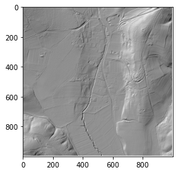
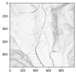
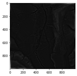
hillshade_arr = default.get_hillshade(dem_arr=dem_arr, resolution_x=dem_res_x, resolution_y=dem_res_y)
plt.imshow(hillshade_arr, cmap='gray')
[10]:
<matplotlib.image.AxesImage at 0x17d9dacb988>
Calculate and save as GeoTIFF in DEM directory:
[11]:
default.save_hillshade(dem_path=dem_path, custom_dir=None, save_float=True, save_8bit=True)
[11]:
1
Multiple directions hillshade
Set parameters:
[12]:
default.mhs_nr_dir = 16
default.mhs_sun_el = 35
Calculate numpy array:
[13]:
mhs_arr = default.get_multi_hillshade(dem_arr=dem_arr, resolution_x=dem_res_x, resolution_y=dem_res_y)
Calculate and save as GeoTIFF in DEM directory:
[14]:
default.save_multi_hillshade(dem_path=dem_path, custom_dir=None, save_float=True, save_8bit=True)
[14]:
1
Simple Local Relief Model (SLRM)
Set parameters:
[15]:
default.slrm_rad_cell = 20
Calculate numpy array:
[16]:
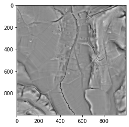
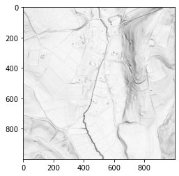
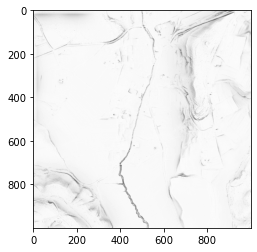
slrm_arr = default.get_slrm(dem_arr=dem_arr)
plt.imshow(slrm_arr, cmap='gray')
[16]:
<matplotlib.image.AxesImage at 0x17d9e2f6808>
Calculate and save as GeoTIFF in DEM directory:
[17]:
default.save_slrm(dem_path=dem_path, custom_dir=None, save_float=True, save_8bit=True)
[17]:
1
Multi-Scale Relief Model (MSRM)
Set parameters:
[18]:
default.msrm_feature_min = 1
default.msrm_feature_max = 5
default.msrm_scaling_factor = 3
Calculate numpy array:
[19]:
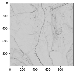
msrm_arr = default.get_msrm(dem_arr=dem_arr, resolution=dem_res_x)
plt.imshow(msrm_arr, cmap='gray')
[19]:
<matplotlib.image.AxesImage at 0x17d9e74b688>
Calculate and save as GeoTIFF in DEM directory:
[20]:
default.save_msrm(dem_path=dem_path, custom_dir=None, save_float=True, save_8bit=True)
[20]:
1
Sky-view factor, Anisotropic sky-view factor, Positive openness
Set parameters:
[21]:
# parameters for all three
default.svf_n_dir = 16
default.svf_r_max = 10
default.svf_noise = 0
# parameters for asvf
default.asvf_dir = 315
default.asvf_level = 1
Calculate numpy array:
[22]:
svf_asvf_opns_dict = default.get_sky_view_factor(dem_arr=dem_arr, resolution=dem_res_x,
                                                 compute_svf=True, compute_asvf=True, compute_opns=True)
[23]:
svf_arr = svf_asvf_opns_dict["svf"]
plt.imshow(svf_arr, cmap='gray')
[23]:
<matplotlib.image.AxesImage at 0x17d9e7d0ac8>
[24]:
asvf_arr = svf_asvf_opns_dict["asvf"]
plt.imshow(asvf_arr, cmap='gray')
[24]:
<matplotlib.image.AxesImage at 0x17d9e8334c8>
[25]:
opns_arr = svf_asvf_opns_dict["opns"]
plt.imshow(opns_arr, cmap='gray')
[25]:
<matplotlib.image.AxesImage at 0x17d9e8b4a08>
Calculate and save as GeoTIFF in DEM directory:
[26]:
default.save_sky_view_factor(dem_path=dem_path, save_svf=True, save_asvf=True, save_opns=True,
                             custom_dir=None, save_float=True, save_8bit=True)
[26]:
1
Negative openness
Set parameters (svf_parameters):
[27]:
default.svf_n_dir = 16
default.svf_r_max = 10
default.svf_noise = 0
Calculate numpy array:
[28]:
neg_opns_arr = default.get_neg_opns(dem_arr=dem_arr, resolution=dem_res_x)
plt.imshow(neg_opns_arr, cmap='gray')
[28]:
<matplotlib.image.AxesImage at 0x17d9e91d1c8>
Calculate and save as GeoTIFF in DEM directory:
[29]:
default.save_neg_opns(dem_path=dem_path, custom_dir=None, save_float=True, save_8bit=True)
[29]:
1
Local dominance
Set parameters:
[30]:
default.ld_min_rad = 10
default.ld_max_rad = 20
default.ld_rad_inc = 1
default.ld_anglr_res = 15
default.ld_observer_h = 1.7
Calculate numpy array:
[31]:
local_dom_arr = default.get_local_dominance(dem_arr=dem_arr)
plt.imshow(local_dom_arr, cmap='gray')
[31]:
<matplotlib.image.AxesImage at 0x17da0cd0f88>
Calculate and save as GeoTIFF in DEM directory:
[32]:
default.save_local_dominance(dem_path=dem_path, custom_dir=None, save_float=True, save_8bit=True)
[32]:
1
Sky illumination
Set parameters:
[33]:
default.sim_sky_mod = "overcast"
default.sim_compute_shadow = 0
default.sim_shadow_dist = 100
default.sim_nr_dir = 32
default.sim_shadow_az = 315
default.sim_shadow_el = 35
Calculate numpy array:
[34]:
sky_illum_arr = default.get_sky_illumination(dem_arr=dem_arr, resolution=dem_res_x)
plt.imshow(sky_illum_arr, cmap='gray')
[34]:
<matplotlib.image.AxesImage at 0x17da0f84e88>
Calculate and save as GeoTIFF in DEM directory:
[35]:
default.save_sky_illumination(dem_path=dem_path, custom_dir=None, save_float=True, save_8bit=True)
[35]:
1
Multi-Scale Topographic Position (MSTP)
Set parameters:
[36]:
default.mstp_local_scale = (1, 5, 1)
default.mstp_meso_scale = (5, 50, 5)
default.mstp_broad_scale = (50, 500, 50)
default.mstp_lightness = 1.2
Calculate numpy array:
[37]:
mstp_arr = default.get_mstp(dem_arr=dem_arr)
Calculate and save as GeoTIFF in DEM directory:
[38]:
default.save_mstp(dem_path=dem_path, custom_dir=None)
[38]:
1